
Handling difficult images
From last week’s post, we know that we can identify images that are particularly difficult using information about classification evenness and the fraction of “nothing here” votes cast. However, the algorithm (and really, all of you volunteers) get the right answer even on hard images most of the time. So we don’t necessary want to just throw out those difficult images. But can we?
Let’s think about two classes of species: (1) the common herbivores and (2) carnivores. We want to understand the relationship between the migratory and non-migratory herbivores. And Ali is researching carnivore coexistence. So these are important classes to get right.
First the herbivores. Here’s a table showing the most common herbivores and our algorithm’s results based on the expert-classified data of about 4,000 images. “Total” is the total number of images that our algorithm classified as that species, and “correct” is the number of those that our experts agreed with.
| species | migratory | total | correct | % correct |
| wildebeest | yes | 1548 | 1519 | 98.1% |
| zebra | yes | 685 | 684 | 100% |
| hartebeest | no | 252 | 244 | 96.8% |
| buffalo | no | 219 | 215 | 98.2% |
| gazelleThomsons | yes | 200 | 189 | 94.5% |
| impala | no | 171 | 168 | 98.3% |
We see that we do quite well on the common herbivores. Perhaps we’d wish for Thomsons gazelles to be a bit higher (Grants gazelles are most commonly mis-classified as Thomsons), but these results look pretty good.
If we wanted to be conservative about our estimates of species ranges, we could throw out some of the images with high Pielou scores. Let’s say we threw out the 10% most questionable wildebeest images. Here’s how we would score. (Note that I didn’t do the zebra, since they’d be at 100% again, no matter how many we dropped.) The columns are the same as the above table, except this time, I’ve listed the threshold Pielou score used to throw out 10% of the images of that species.
| species | Pielou cutoff | total | correct | % correct |
| wildebeest | 0.60 | 1401 | 1389 | 99.1% |
| hartebeest | 0.73 | 228 | 223 | 97.8% |
| buffalo | 0.76 | 198 | 198 | 100% |
| gazelleThomsons | 0.72 | 180 | 175 | 97.2% |
| impala | 0.86 | 155 | 153 | 98.7% |
We do quite a bit better with our Thomsons gazelle and increase the accuracy of all the other species at least a little. But do we sacrifice anything throwing out data like that? If wildebeest make up a third of our images and we have a million images, then we’re throwing away 33,000 images(!), but we still have another 300,000 left to do our analyses. One thing we will look at in the future is how much dropping the most questionable images affects estimates of species ranges. I’m guessing that for wildebeest it won’t be much.
What if we did the same thing for Thomsons gazelle or impala? We would expect about 50,000 images of each of those per million images. Throwing out 5,000 images still leaves us with 45,000, which seems like it might be enough for many analyses.
Now let’s look at the carnivore classifications from the expert-validated data set:
| species | total | correct | % correct |
| hyenaSpotted | 55 | 55 | 100% |
| lionFemale | 18 | 18 | 100% |
| cheetah | 6 | 6 | 100% |
| serval | 6 | 6 | 100% |
| leopard | 3 | 3 | 100% |
| jackal | 2 | 2 | 100% |
| lionMale | 1 | 1 | 100% |
| aardwolf | 1 | 1 | 100% |
| batEaredFox | 1 | 0 | 0% |
| hyenaStriped | 1 | 0 | 0% |
Wow! You guys sure know your carnivores. The two wrong answers were the supposed bat-eared fox that was really a jackal and the supposed striped hyena that was really an aardwolf. These two wrong answers had high Pielou scores: 0.77 and 0.83 respectively.
Judging by this data set, about 2.5% of all images are carnivores, which gives us about 25,000 carnivore images for every million we collect. That’s a lot of great data on these relatively rare animals! But it’s not so much that we want to throw any of it away. Fortunately, we won’t have to. We can use the Pielou score to have an expert look at the most difficult images.
Let’s say Ali wants to be very confident of her data. She can choose the 20% most difficult carnivore images — which is only about 5,000 per million images, and she can go through them herself. Five thousand images is nothing to sneeze at, of course, but the work can be done in a single day of intense effort.
In summary, we might be able to throw out some of the more difficult images (based on Pielou score) for the common herbivores without losing much coverage in our data. Further analyses are needed, though, to see if doing so is worthwhile and whether we lose anything by throwing out so many correct answers. For carnivores, the difficult images can be narrowed down sufficiently that an expert can double-check them by hand.
Certainty score
Back in June, I wrote about algorithms I was working on to take the volunteer data and spit out the “correct” classification of for each image. First, I made a simple majority-rules algorithm and compared its results to several thousand classifications done by experts. Then, when the algorithm came up with no answer for some of the images (because there were no answers in the majority), I tried a plurality algorithm, which just looked to see which species got the most votes, even if it didn’t get more than half the votes. It worked well, so I’m using the plurality algorithm going forward.
One of the things I’ve been curious about is whether we can detect when particular images are “hard.” You know what I mean by hard: animals smack up in front of the camera lens, animals way back on the horizon, animals with just a tip of the ear or a tuft of tail peeking onto the image from one side, animals obfuscated by trees or the dark of night.
So how can we judge “hard”? One way is to look at the “evenness” of the volunteer votes. Luckily, in ecology, we deal with evenness a lot. We frequently want to know what species are present in a given area. But we also want to know more than that. We want to know if some species are very dominant in that area or if species are fairly evenly distributed. For example, in a famous agricultural ecology paper*, Cornell entomologist Richard Root found that insect herbivore (pest) species on collard greens were less even on collards grown in a big plot with only other collards around versus on those grown in a row surrounded by meadow plants. In other words, the insect species in the big plot were skewed toward many individuals of just a few species, whereas in the the meadow rows, there were a lot more species with fewer individuals of each species.
We can adopt a species evenness metric called “Pielou’s evenness index” (which, for you information theorists, is closely related to Shannon entropy.)
[An aside: I was surprised to learn that this index is named for a woman: Dr. Evelyn Chrystalla Pielou. Upon reflection, this is the first time in my 22 years of formal education (in math, computer science, and ecology) that I have come across a mathematical term named for a woman. Jacqueline Gill, who writes a great paleo-ecology blog, has a nice piece honoring Dr. Pielou and her accomplishments.]
Okay, back to the Pielou index: we can use it to judge how even the votes are. If all the votes are for the same species, we can have high confidence. But if we have 3 votes for elephant and 3 votes for rhino and 3 votes for wildebeest and 3 votes for hippo, then we have very low confidence. The way the Pielou index works out, a 0 means all the votes are for the same species (high skew, high confidence) and a 1 means there are at least two species and they all got the same number of votes (high evenness, low confidence). Numbers in between 0 and 1 are somewhere between highly skewed (e.g. 0.2) and really even (e.g. 0.9).
Another way we could measure the difficulty of an image is to look at how many people click “nothing here.” I don’t like it, but I suspect that some people use “nothing here” as an “I don’t know” button. Alternatively, if animals are really far away, “nothing here” is a reasonable choice. We might assume that the percentage of “nothing here” votes correlates with the difficulty of the image.
I calculated the Pielou evenness index (after excluding “nothing here” votes) and the fraction of “nothing here” votes for the single-species images that were classified by experts. And then I plotted them. Here I have the Pielou index on the x-axis and the fraction of “nothing here” votes on the y-axis. The small pink dots are the 3,775 images that the algorithm and the experts agreed on, the big blue dots are the 84 images that the plurality algorithm got wrong, and the open circles are the 29 images that the experts marked as “impossible.” (Click to enlarge.)
 And sure enough, we see that the images the algorithm got wrong had relatively high Pielou scores. And the images that were “impossible” had either high Pielou scores or a high fraction of “nothing here” votes (or both). I checked out the four anomalies over on the left with a Pielou score of zero. All four were unanimously voted as wildebeest. For the three “impossibles,” both Ali and I agree that wildebeest is a reasonable answer. But Ali contends that the image the algorithm got wrong is almost certainly a buffalo. (It IS a hard image, though — right up near the camera, and at night.)
So we do seem to be able to get an idea of which images are hardest. But note that there are a lot more correct answers with high Pielou scores and high “nothing here” fractions than errors or “impossibles”. We don’t want to throw out good data, so we can’t just ignore the high-scorers. But we can attach a measure of certainty to each of our algorithm’s answers.
—
Plurality algorithm
On Wednesday, I wrote about how well the simple algorithm I came up with does against the experts. The algorithm looks for species that have more than 50% of the votes in a given capture (i.e. species that have a majority). Commenter Tor suggested that I try looking at which species have the most votes, regardless of whether they cross the 50% mark (i.e. a plurality). It’s a great idea, and easy to implement because any species that has more than 50% of the vote ALSO has the plurality. Which means all I have to do is look at the handful of captures that the majority algorithm had no answer for.
You can see why it might be a good idea in this example. Say that for a particular capture, you had these votes:
| 10 | impala |
| 4 | gazelleThomsons |
| 4 | dikDik |
| 3 | bushbuck |
You’d have 21 votes total, but the leading candidate, impala, would be just shy of the 11 needed to have a majority. It really does seem like impala is the likely candidate here, but my majority algorithm would come up with “no answer” for this capture.
So I tried out Tor’s plurality algorithm. The good news is that 57% of those “no answers” got the correct answer with the plurality algorithm. So that brings our correct percentage from 95.8% to 96.6%. Not bad! Here’s how that other 3.4% shakes out:
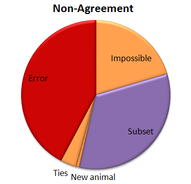
So now we have a few more errors. (About a quarter of the “no answers” were errors when the plurality algorithm was applied.) And we’ve got a new category called “Ties”. When you look for a plurality that isn’t over 50%, there can be ties. And there were. Five of them. And in every case the right answer was one of the two that tied.
And now, because it’s Friday, a few images I’ve stumbled upon so far in Season 5. What will you find?


Algorithm vs. Experts
Recently, I’ve been analyzing how good our simple algorithm is for turning volunteer classifications into authoritative species identifications. I’ve written about this algorithm before. Basically, it counts up how many “votes” each species got for every capture event (set of images). Then, species that get more than 50% of the votes are considered the “right” species.
To test how well this algorithm fares against expert classifiers (i.e. people who we know to be very good at correctly identifying animals), I asked a handful of volunteers to classify several thousand randomly selected captures from Season 4. I stopped everyone as soon as I knew 4,000 captures had been looked at, and we ended up with 4,149 captures. I asked the experts to note any captures that they thought were particularly tricky, and I sent these on to Ali for a final classification.
Then I ran the simple algorithm on those same 4,149 captures and compared the experts’ species identifications with the algorithm’s identifications. Here’s what I found:
 For a whopping 95.8% of the captures, the simple algorithm (due to the great classifying of all the volunteers!) agrees with the experts. But, I wondered, what’s going on with that other 4.2%. So I had a look:
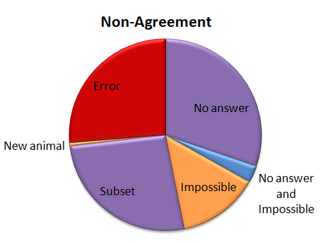 Of the captures that didn’t agree, about 30% were due to the algorithm coming up with no answer, but the experts did. This is “No answer” in the pie chart. The algorithm fails to come up with an answer when the classifications vary so much that there is no single species (or combination if there are multiple species in a capture) that takes more than 50% of the vote. These are probably rather difficult images, though I haven’t looked at them yet.
Another small group — about 15% of captures was marked as “impossible” by the experts. (This was just 24 captures out of the 4,149.) And five captures were both marked as “impossible” and the algorithm failed to come up with an answer; so in some strange way, we might consider these five captures to be in agreement.
Just over a quarter of the captures didn’t agree because either the experts or the algorithm saw an extra species in a capture. This is labeled as “Subset” in the pie chart. Most of the extra animals were Other Birds or zebras in primarily wildebeest captures or wildebeest in primarily zebra captures. The extra species really is there, it was just missed by the other party. For most of these, it’s the experts who see the extra species.
Then we have our awesome, but difficulty-causing duiker. There was no way for the algorithm to match the experts because we didn’t have “duiker” on the list of animals that volunteers could choose from. I’ve labeled this duiker as “New animal” on the pie chart.
Then the rest of the captures — just over a quarter of them — were what I’d call real errors. Grant’s gazelles mistaken for Tommies. Buffalo mistaken for wildebeest. Aardwolves mistaken for striped hyenas. That sort of thing. They account for just 1.1% of all the 4,149 captures.
I’ve given the above Non-agreement pie chart some hideous colors. The regions in purple are what scientists call Type II errors, or “false negatives.” That is, the algorithm is failing to identify a species that we know is there — either because it comes up with no answer, or because it misses extra species in a capture. I’m not too terribly worried about these Type II errors. The “Subset” ones happen mainly with very common animals (like zebra or wildebeest) or animals that we’re not directly studying (like Other Birds), so they won’t affect our analyses. The “No answers” may mean we miss some rare species, but if we’re analyzing common species, it won’t be a problem to be missing a small fraction of them.
The regions in orange are a little more concerning; these are the Type I errors, or “false positives.” These are images that should be discarded from analysis because there is no useful information in them for the research we want to do. But our algorithm identifies a species in the images anyway. These may be some of the hardest captures to deal with as we work on our algorithm.
And the red-colored errors are obviously a concern, too. The next step is to incorporate some smarts into our simple algorithm. Information about camera location, time of day, and identification of species in captures immediately before or following a capture can give us additional information to try to get that 4.2% non-agreement even smaller.
